Mathematics Statistics, Image Processing Analysis, Informatics
- Mathematics relevant to medical physics
- Statistics and biostatistics
- Medical image analysis and processing
- Observer performance and ROC analysis Informatics
Mathematics relevant to medical physics
Log/Ln rules:
$\log(A \times B) = \log(A) + \log(B)$
$\log(A/B) = \log(A) - \log(B)$
$\log(A^B) = B \log (A)$
Exponentials
$\int{e^{a x} dx} = \tfrac{1}{a} e^{a x} + C$
Product rule: $\frac{d}{dx}(f(x)\cdot g(x)) = f'(x)g(x) + f(x)g'(x)$
Chain rule: $\frac{d}{dx}(f(g(x)) = f'(g(x))g'(x)$
Statistics and biostatistics
mean = $\bar{x} = \sum{x_i} /n$
median = middle number in ordered data points
standard deviation = $\sigma = \sqrt{ \frac{\sum{(x_i-\mu)^2}}{N} }$ where $\mu$ is the mean and $x_i$ is each of $N$ data points
coefficient of variation (cov) = $\sigma / \mu$ (relative standard deviation)
variance = $\sigma^2$
standard error: measure of accuracy of a measurement. Standard deviation of a sampling distribution.
Bayes' theorem: Probability of an event given prior knowledge of related conditions
$P(A\mid B)=\frac{P(B\mid A)\,P(A)}{P(B)}$
Probability of event A given that B is true depends on probability of A, of B, and of B given that A is true.
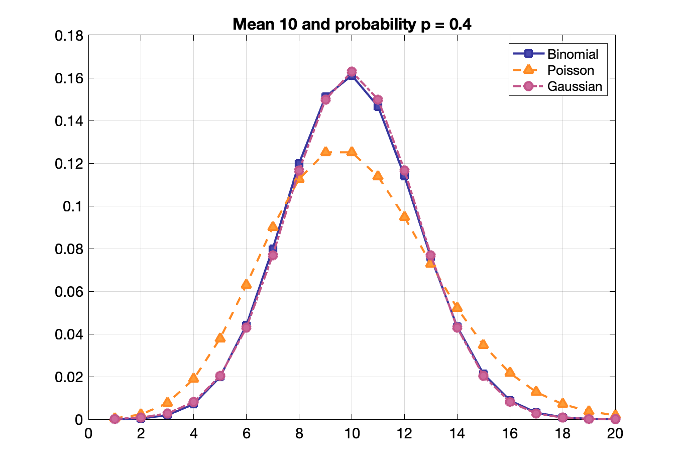
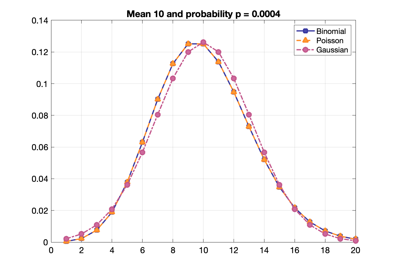
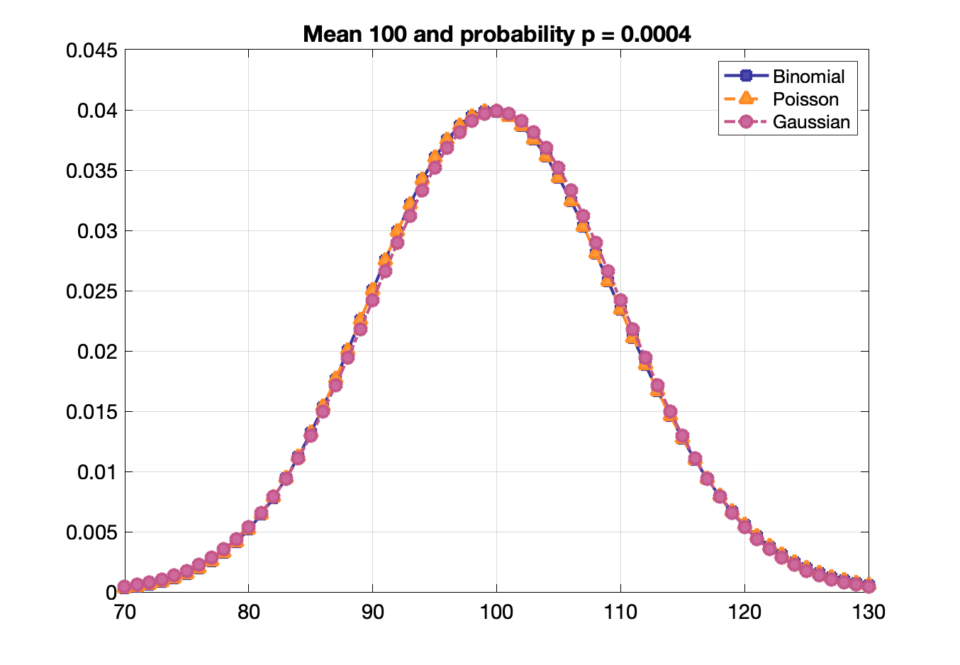
Binomial, Poisson, Gaussian distribution functions
Binomial: probability of getting exactly $x$ successes in $N$ trials given a single trial probability $p$
$P(x) = \frac{N!}{x!(N-x)!}p^x(1-p)^{N-x}$
$\bar{x} = pN$ and $\sigma = \sqrt{pN(1-p)}$ and for small p: $\approx \sqrt{pN} \approx \sqrt{\bar{x}}$
Useful when there is high counting efficiency.
Poisson statistics: probability of a given number of events occurring in a fixed interval of time or space if these events occur with a known constant rate, e.g., radioactive decay
Probability of $n$ events given an average of $\lambda$ events: $P = \frac{\lambda^n\,e^{-\lambda}}{n!}$
Expected value = $\lambda$ and variance = $\lambda$
Approximate standard deviation for a single measurement: $\sigma \approx \sqrt{x}$
Fractional error (cov): $\sigma/x \approx 1/\sqrt{x}$
E.g. fractional error of 40,000 counts ~ 1/sqrt(40,000) = 1/200 = 5%
Useful for low detection efficiency and when $p$ or $n$ is not known directly.
Gaussian: normally distributed
$\text{PDF} = \frac{1}{\sqrt{2\pi\sigma^2}} e^{-\frac{(x-\mu)^2}{2 \sigma^2}}$
Standard deviation: (σ) For a normal distribution, 68.3% of measurements are within 1 σ, 95.5% within 2 σ, 99.7 within 3 σ.
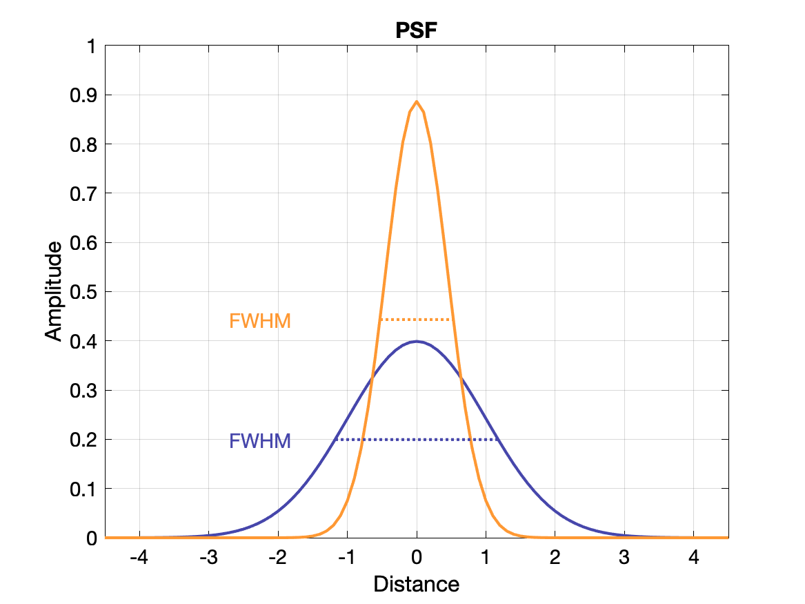
Full width half max: $\text{FWHM} = 2.355 \sigma$
Poisson, binomial and Gaussian distributions become identical when $p$ is small and mean is large.
Confidence interval: Interval for the probability of containing the true mean. E.g., there is a 68.27% probability that the true mean is within 1 σ of a measurement and 95.45% probability it is within 2 σ.
95% confidence for measurement of 40,000 cts is 40,000 ± 1.96 σ = 40,000 ± 392 cts. Thus the 95% confidence interval is from 39,608 to 40,392 cts.
| Probability that mean is within % | Interval around measurement |
| 50 | ±0.674 σ |
| 68.3 | ±1 σ |
| 90 | ±1.64 σ |
| 95 | ±1.96 σ |
| 95.5 | ±2 σ |
| 99 | ±2.58 σ |
| 99.7 | ±3 σ |
(Spatial) Resolution
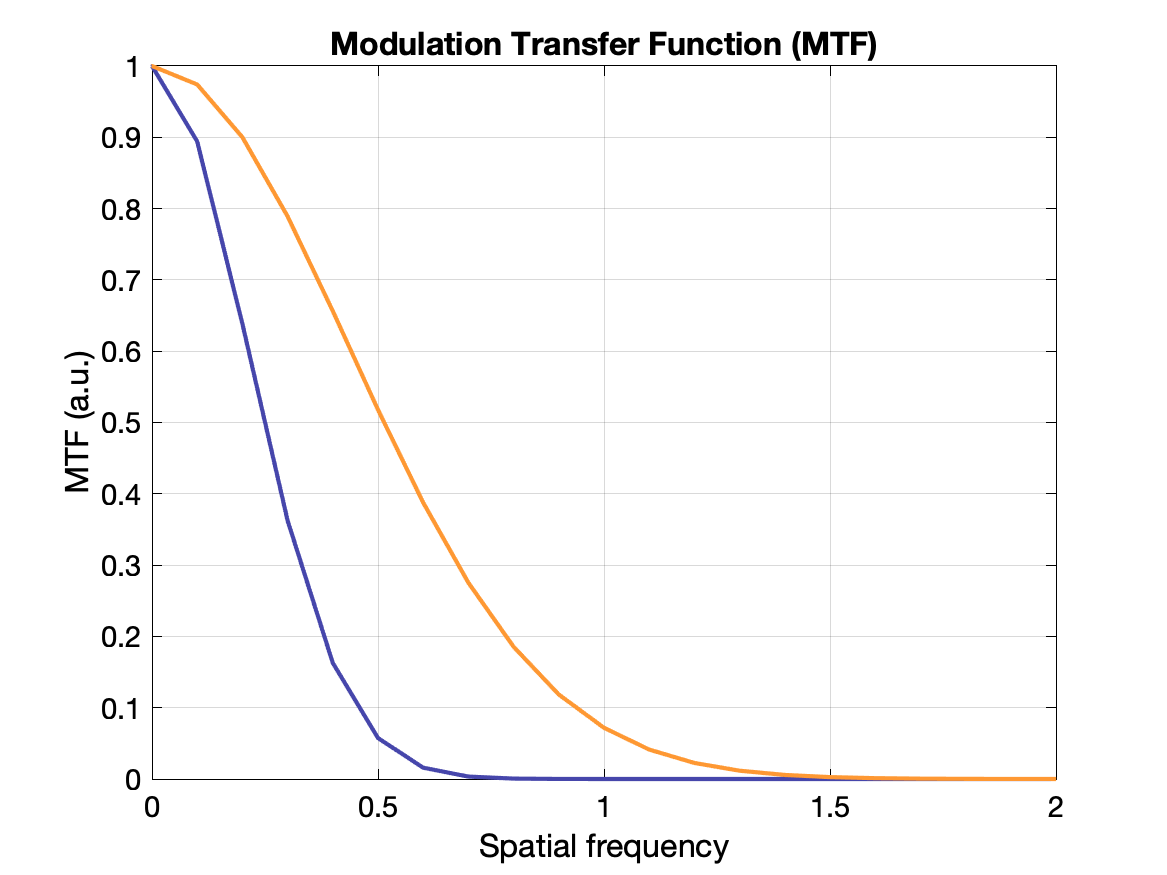
Spatial resolution is often measured with a point source and in images exhibits a gaussian distribution of intensity: the point spread function (PSF). The value of the resolution is typically given as the FWHM of the PSF, where FWHM = 2.355σ.
Another way to display the response of a system to spatial frequency is to create a modulation transfer function (MTF) - essentially how well the system can recover the true intensity for a range of frequencies. An ideal system would have MTF = 1 for all frequencies, but it more typically falls off gradually as the frequency increases. The MTF is calculated as the Fourier transform of the PSF. See plots below.
Modulation: $M = (I_{max} - I_{min}) / (I_{max} + I_{min})$ where $I$s are the min and max radiation intensities in the test pattern. If $I_{min} = I_{max}$ there is no contrast. If $I_{min}=0$ there is maximum contrast.
$\text{MTF}(k) = M_{out}(k) / M_{in}(k)$ where $M_{out}$ is the modulation of the output (image) and $M_{in}$ is the modulation of the original pattern for each frequency $k$.
Propagation of error
If the standard deviation of x is σ, the standard deviation of x/c is σ/c so long as c does not have random error.
Two numbers with error are added/subtracted: $x_1 + x_2 \rightarrow \sigma = \sqrt{\sigma_1^2 + \sigma_2^2}$
Other cases: ${\displaystyle s_{f}={\sqrt {\left({\frac {\partial f}{\partial x}}\right)^{2}s_{x}^{2}+\left({\frac {\partial f}{\partial y}}\right)^{2}s_{y}^{2}+\left({\frac {\partial f}{\partial z}}\right)^{2}s_{z}^{2}+\cdots }}}$
Random errors: unknown, unpredictable (stochastic, noise). Usually have a gaussian distribution.
Systematic errors: incorrect measurements that are affect measurements in the same way each time. E.g., problems with the measuring instrument, Can be an offset error (e.g., instrument not zero when quantity is zero) or multiplicative/scale factor (e.g. instrument does not measure linearly when it should).
Precision: How much the individual values deviate around the true value.
Accuracy: How close the measured value is to the true value.
Random errors limit precision but less so accuracy. Systematic errors might not affect precision but usually affect accuracy.
Linear regression
Model relationship of dependent variables to explanatory variables. Parameters of the model are estimated from data, typically using the least squares method.
Least squares: minimize the square difference between the data and the model estimation when varying input parameters.
Comparative tests
- Chi-square test
- Valid when test statistic follows a chi-square distribution under the null hypothesis
- Pearson's chi-squared test for categorical data: test how likely observed differences between sets arises from chance
- $\chi^2 = \sum_{i=1}^n{\frac{(O_i - E_i)^2}{E_i}}$ where $O_i$ is number of observations of type $i$ and $E_i = Np_i$ is expected count of type $i$ for $N$ observations in population $p_i$.
- Can be used to calculate p-value by comparing value to a chi-squared distribution given the degrees of freedom.
- Sensitive to distribution of categories (too few in one category) and too large sample size
- Useful webpage from Kent State University on Chi-square tests
- t-test (Student t-test)
- Used to asses if any difference between sample mean and expected population (true) mean is due only to chance
- One sample: sample mean different from hypothesized mean
- $t = \frac{\bar{x} - \mu}{s/\sqrt{n}}$, where $\bar{x}$ is sample mean, $\mu$ is hypothesized mean, $s$ is the sample standard deviation, and $n$ is sample size
- Assumes $\bar{x}$ follows normal distribution
- Paired sample: sample one mean different from sample two mean, for paired samples
- $t={\frac {{\bar {X}}_{D}-\mu _{0}}{s_{D}/{\sqrt {n}}}}$ where ${\bar {X}}_{D}$ and $s_D$ are the average and standard deviation of the differences between pairs
- Independent sample: sample one mean different from sample two mean, for two independent groups
- $ t={\frac {{\bar {X}}_{1}-{\bar {X}}_{2}}{s_{p}{\sqrt {\frac {2}{n}}}}}$ where $s_{p}={\sqrt {\frac {s_{X_{1}}^{2}+s_{X_{2}}^{2}}{2}}}$ is the pooled standard deviation. Can also be weighted sample size when unequal.
- Set theory (multiple testing)
- Multiple comparisons problem / look-elsewhere effect: the more comparisons that are done, the increased likelihood of finding one significant erroneously.
- Family-wise error rate: ${\bar {\alpha }}=1-\left(1-\alpha _{\{{\text{per comparison}}\}}\right)^{m}$ where $m$ is the number of independent comparisons.
- Bonferroni correction: $\alpha _{\mathrm {\{per\ comparison\}} }={\alpha }/m$
Counting statistics
See also poisson statistics above, where $\sigma = \sqrt{N}$
Measurement with background is the gross counts minus the background counts: $N_s = N_g - N_b$ and $\sigma_s = \sqrt{N_g + N_b}$ and fractional standard deviation (cov) is $\sigma_F(N_s) = \dfrac{\sqrt{N_g+N_b}}{N_g - N_b}$
Minimum net counts that can be detected with 99.7% confidence (3σ): $N_g - N_b > 3\sigma(N_g - N_b) = 3 \sqrt{N_g + N_b}$
Propagation of errors in count rates:
$N$ counts over time $t$ gives a count rate $R = N/t$.
Generally assume that $t$ has small enough uncertainty to be considered a constant.
Uncertainty in counting rate: $\sigma_R = \dfrac{\sigma_x}{t} = \dfrac{\sqrt{N}}{t} = \sqrt{\dfrac{R}{t}}$
Minimum detectable activity - must have sample count rate three standard deviations above background count rate: $\text{MDA} = 3\sigma_R = 3 \sqrt{R_B/t}$
Medical image analysis and processing
Nyquist frequency: $f = 1/(2\Delta r)$ where $\Delta r$ is the sampling rate. Sample rate must be 2x highest frequency in signal to avoid aliasing.
Rule of thumb: $\Delta r \leq FWHM/3$
Angular sampling for diameter D: $N_{views} \geq \pi D / 2\Delta r$
Coefficient of variation (COV) = $\sigma / N$ where $\sigma$ is standard deviation and $N$ is average number of counts. For Poisson statistics, $\sigma = \sqrt(N)$
Intrinsic efficiency: measured counts / incident counts (# of quanta)
Extrinsic efficiency: measured counts / source counts (# of quanta)
1 kilobyte (KB) = 1024 bytes = 210 bytes
1 megabyte (MB) = 1024 KB = 220 bytes
1 gigabyte (GB) = 1024 MB = 230 bytes
1 terabyte (TB) = 1024 GB = 240 bytes
Observer performance and ROC analysis Informatics
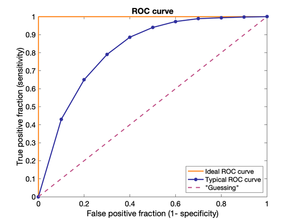 ROC = Receiver Operating Characteristic
Plot of Sensitivity vs 1-Specificity = true positive fraction (TPF) vs false positive fraction (FPF)
Useful for demonstrating the diagnostic ability of a test for various discrimination thresholds (trading off between TPF and FPF). 45-degree diagonal equivalent of guessing, curve ideally lies high above.
Area under the ROC curve can be used as a single reporting parameter.
0 = all wrong, 1 = all right, 0.5 = "guessing".
ROC studies require a ground truth measurement (e.g. biopsy to confirm imaging results)
Sensitivity: true positive fraction, probability of detection, is the proportion of actual positives that are correctly identified
TPF = TP / P = TP / (TP + FN)
Specificity: true negative fraction, is proportion of actual negatives that are correctly identified
TNF = TN / N = TN / (TN + FP)
Precision (positive predictive value): Fraction of positives that are true positives: TP / (TP + FP)
Negative predictive value: Fraction of negatives that are true negatives: TN / (TN+FN)
False negative rate: Fraction of false negatives over all positives: FN / (FN+TP)
False positive rate: Fraction of false positives over all negatives: FP / (FP+TN)
Accuracy: fraction of all events that are correctly identified
A = (TP + TN) / (TP + FP + TN + FN)
Critical level: threshold where probability of false positive is less than a probability α
